Bolster’s detection engine relies heavily on deep learning to detect fraud in real-time. When combined with fast image matching it gives us a great balance between speed and accuracy
When we scan a webpage, we take a high-resolution screenshot of it. Our fast image matching algorithm looks at the screenshot of a webpage and matches it with the ones stored in a database. When we started researching for an image matching algorithm, we came with two criteria. It needs to be fast – matching an image under 15 milliseconds, and it needs to be at least 90% accurate, causing the least number of false positives. Satisfying both these criteria helped us scan over a billion URLs and match hundreds of millions of screenshots.
In the first part of the blog, we discuss several feature detection algorithms we experimented with, and in the second, we discuss how these features can be matched at scale.
Feature Detection Algorithms
In this section, we discuss feature detection algorithms that we tried out. All these matching algorithms are available as part of the opencv-python.
1. SIFT: Scale-Invariant Feature Transform
SIFT, proposed by David Lowe in this paper (link), has four main steps which are feature point detection, localization, orientation assignment, and feature descriptor generation.
SIFT is not free to use.
2. SURF: Speeded Up Robust features
A major disadvantage of SIFT is that it is slow. SURF added a lot of features to improve the speed of the SIFT algorithm in every step. SURF is good at handling images with blurring and rotation but not good at handling viewpoint change and illumination change. SURF is better than SIFT in rotation invariant, blur, and warp transform. SIFT is better than SURF in different scale images. SURF is three times faster than SIFT because of the use of integral image and box filters. [1]
Just like SIFT, SURF is not free to use.
3. ORB: Oriented FAST and Rotated BRIEF
ORB algorithm was proposed in the paper “ORB: An efficient alternative to SIFT or SURF.” The paper claims that ORB is much faster than SURF and SIFT, and its performance is better than SURF.
Unlike the other two, ORB is free to use and is also available as part of the opencv-python package. Here is a quick and simple implementation of ORB.
import cv2
img = cv2.imread(image.jpg’,0)
orb = cv2.ORB()
keypoint = orb.detect(img,None)
keypoint, des = orb.compute(img, keypoint)


4. AKAZE: Accelerated KAZE
The feature description performed by AKAZE is based on a Modified Local Difference Binary that uses a gradient to intensity information. This makes the descriptors robust to changes in scale. ORB is faster to compute than AKAZE and the processing time of AKAZE quickly rises with increasing image resolution. However, after filtering the matches and removing outliers, AKAZE presents a more significant number of correct matches when compared with ORB. AKAZE shows a better compromise between speed and performance than ORB for images with low resolution. [4]
AKAZE is also available as part of the opencv-python package. Here is a quick and simple implementation.
import cv2 as cv
img = cv.imread(‘image.jpg’)
akaze = cv.AKAZEcreate()
kp, descriptor = akaze.detectAndCompute(img, 0)
img2=cv.drawKeypoints(img, kp, img)
cv.imwrite(‘AKAZ.jpg’, img2)
If you are interested in comparing different descriptor matching, here is a comparison paper [2]. Here are some results of AKZE and ORB matching on some different internet pages.

We decided to move forward with ORB feature detection its performance is much better than AKAZE with high resolution images.
Image matching at Scale
In this section, we discuss how we matched the features we extracted in the Feature detection algorithms section. All these matching algorithms are available as part of the opencv-python.
1. Brute force matching
Brute-Force matching takes the extracted features (/descriptors) of one image, matches it with all extracted features belonging to other images in the database, and returns the similar one. This matching algorithm is very slow and the time taken to match linearly increases with the number of features being added. This results in higher computational costs.
kp1, des1 = orb.detectAndCompute(img1,None)
kp2, des2 = orb.detectAndCompute(img2,None)
bf = cv.BFMatcher()
matches = bf.knnMatch(des1,des2,k=2)
2 . Flann
FLANN (Fast Library for Approximate Nearest Neighbors) is an image matching algorithm for fast approximate nearest neighbor searches in high dimensional spaces. These methods project the high-dimensional features to a lower-dimensional space and then generate the compact binary codes. Benefiting from the produced binary codes, fast image search can be carried out via binary pattern matching or Hamming distance measurement, which dramatically reduces the computational cost and further optimizes the efficiency of the search.
kp1, des1 = sift.detectAndCompute(img1,None)
kp2, des2 = sift.detectAndCompute(img2,None)
FLANNINDEXKDTREE = 1
indexparams = dict(algorithm = FLANNINDEXKDTREE, trees = 5)
searchparams = dict(checks=50)
flann = cv.FlannBasedMatcher(indexparams,searchparams)
matches = flann.knnMatch(des1,des2,k=2)
3. HNSW
The HNSW builds a hierarchical graph incrementally [3], an approximate K-nearest neighbor descriptor based on small-world graphs with hierarchy. This model is fully graph-based, without any additional search structures that have a high recall. Each node in the graph is linked to the other node in the closest space. The hierarchical structure in HNSW helps to skip far away from neighbors on the low dimensional case. The speed-efficiency over the approaches without hierarchy support is around two times to its best. The problem of HNSW is the cures of dimensionality that can not address this issue. Follow the HNSW Github. link
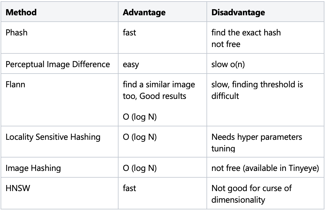
The comparison of different methods:

FLANN vs HNSW:
We compared the results of both algorithms, HNSW and FLANN, in terms of speed. We need to find a balance between speed and accuracy for the model. HNSW is working well for both of them for us. HNSW is faster than Flann, and we decided to use HNSW for image matching.

Results:
Here are the results of the image matching using HNSW. We compared different distance thresholds for HNSW. Time is in milliseconds.

References:
[1] Mistry, Darshana, and Asim Banerjee. “Comparison of feature detection and matching approaches: SIFT and SURF.” GRD Journals-Global Research and Development Journal for Engineering 2.4 (2017): 7-13.
[2] Tareen, Shaharyar Ahmed Khan, and Zahra Saleem. “A comparative analysis of sift, surf, kaze, akaze, orb, and brisk.” 2018 International conference on computing, mathematics and engineering technologies (iCoMET). IEEE, 2018.
[3] Malkov, Yu A., and Dmitry A. Yashunin. “Efficient and robust approximate nearest neighbor search using hierarchical navigable small world graphs.” IEEE transactions on pattern analysis and machine intelligence 42.4 (2018): 824-836.
[4]Roosab, Daniel R., Elcio H. Shiguemori, and Ana Carolina Lorenac. “Comparing ORB and AKAZE for visual odometry of unmanned aerial vehicles.” (2016).
Learn more about Bolster’s Brand Protection, Fraud Prevention, and Phishing & Scam solutions.
Request a Free Trial today.


